Principles
Classic Principle of TCSPC
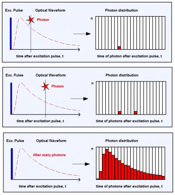
Time correlated single photon counting (TCSPC) detects single photons of a periodic light signal and determines the times of the photons after the excitation pulses.
The pulse repetition rate of the signal is much higher than the photon detection rate. Therefore, the detection of several photons per signal period is extremely unlikely. Only a single photon per signal period needs to be considered. Under these conditions, the time of this photon can be determined at extremely high resolution.
From the times of the individual photons TCSPC builds up the distribution of the photons over the time after the excitation pulse. The photon distribution represents the waveform of the optical signal, see figure on the right.
Outstanding Features
TCSPC has a number of other outstanding features. First, it achieves a near-ideal photon efficiency: Every photon seen by the detector ends up in the photon distribution, and thus contributes to the result.
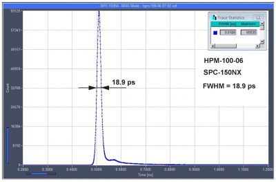
Second, TCSPC reaches an extremely high time resolution. The resolution is not limited by the single-photon response uf the detector, as it is the case for analog-recording techniques. Instead, the resolution is given by the transit-time jitter of the electrons in the detector. This can be by a factor of 10 to 50 smaller than the width of the single-photon pulse. As an example, the bh TCSPC devices achieve an instrument-response function (IRF) of less than 20 ps full width at half maximum with a hybrid detector that has a single-photon response of about 1 ns width.
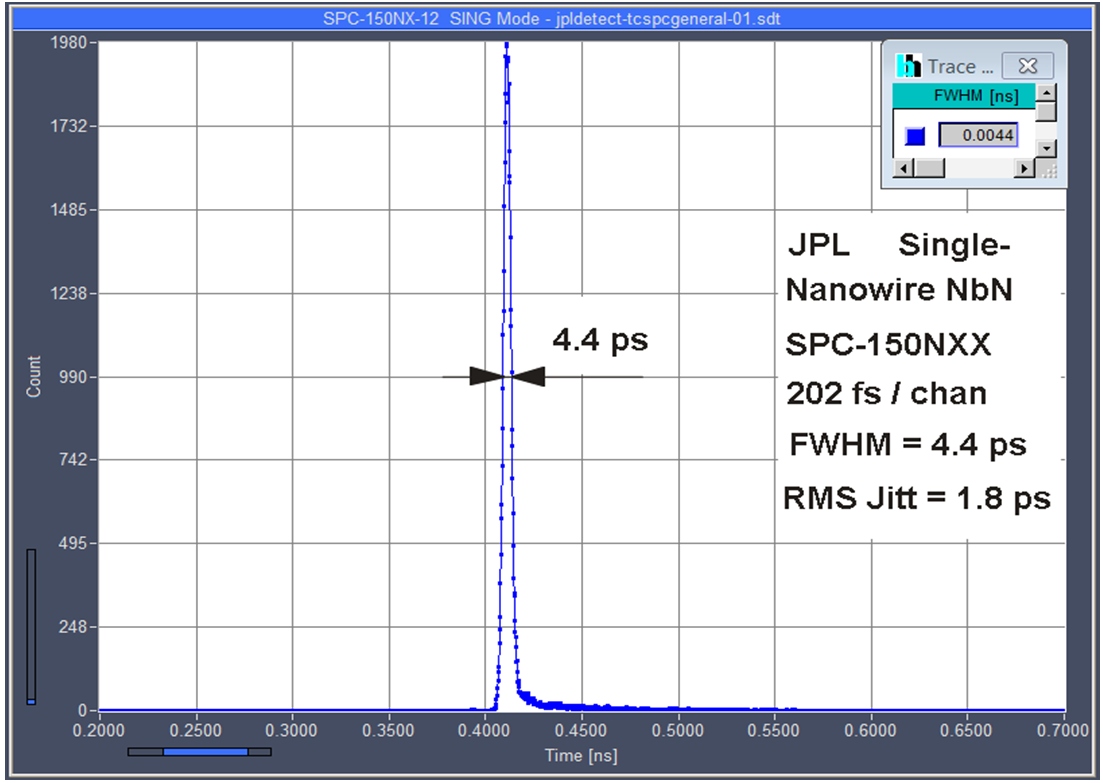
Third, with the bh TCSPC devices even the fastest IRF can be sampled at a point density that satisfies the Nyquist condition. With time-channel widths down to 203 femtoseconds being available, even the last bit of temporal information can be exctracted from the recorded signals.
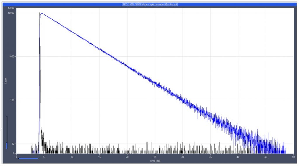
Fourth, TCSPC reaches an extremely high dynamic range, and an extremely high linearity. In fact, the dynamic range is only limited by the ratio of the rate of the signal photons and the background count rate.

The high dynamic range in combination with the high linearity makes it possible to analyse multi-exponential fluorescence-decay processes. This is an extraordinarily important feature for applications in life sciences: The information in these applications is not directly in the apparent liftime of the fluorescence decay but in the composition of the decay, i.e. in the liftimes and the amplitudes of the decay components. Please see The bh TCSPC Handbook for details.
Advanced TCSPC Techniques
The most intriguing feature of TCSPC is, however, that the recording process can be made multi-dimensional. That means the TCSPC device records photon distributions not only over the times of the photons in a fluorescence decay but, simultanneously, over the wavelength of the photons, the wavelength of the excitation, the time after a stimulation of the sample, over the spatial coordinates of an image area where the photons are coming from, or any other parameter that can be determined for the individual photon simultaneously with their times. These advanced TCSPC principles have opened the way to entirely new classes of experiments. Please see ‘Multi-Dimensional TCSPC’, ‘TCSPC FLIM’, ‘Multi-Wavelength FLIM’, and ‘Simultaneous FLIM/PLIM’. Please see also ‘The bh TCSPC Technique‘ (a 40-page brochure) and ‘The bh TCSPC Handbook’.
Pile Up
As an argument against TCSPC it is often stated that the technique is plagued by the ‘Pile-Up-Effect’. Pile-up means the detection of a second photon in the same signal period with a previous one, causing a distortion of the recorded optical waveform. Please don’t get confused by such statements.
The commonly stated pile-up limit of 0.1% of the excitation rate is wrong. The correct value is 0.1 x Excitation Rate, or 10% of it. This is 100 times more than commonly believed! The limit of 0.1% stems from a typo in the TCSPC literature of the late 1970s. Since then, the mistake cas been copied uncritically again and again. With the correct value of the pile-up limit, the maximum count rate for 80 MHz repetition rate is 8 MHz (8×10⁶ photons per second). This is at least 10 times more than typical FLIM samples can deliver without photo-induced changes in their molecular structure.
A deriviation of the correct size of the pile-up error and the conclusion of its irrelevance for TCSPC and TCSPC FLIM can be found in [1] and [2]. How deeply the misconception of pile-up is fixed in the minds of the users becomes evident from the fact that [1] is constantly cited as a proof of the alledgedly devastating effect of pile-up on TCSPC FLIM. In fact, it proofs the opposite. Therefore, make sure that you cite the reference in the correct context. If you carelessly copy the mistake you show that you either have stolen the reference from another paper, or that you were unable to grasp the point of it – which even sub-average intelligence should be able to.
Practical Implementation
For practical implementation please see Lasers, Detectors and TCSPC Devices on this website, and ‘The bh TCSPC Handbook’, chapter ‘Implementation of the bh TCSPC technique’.
References
[1] W. Becker, Advanced Time-correlated Single Photon Counting Techniques, Springer, 2005
[2] W. Becker, The bh TCSPC Handbook